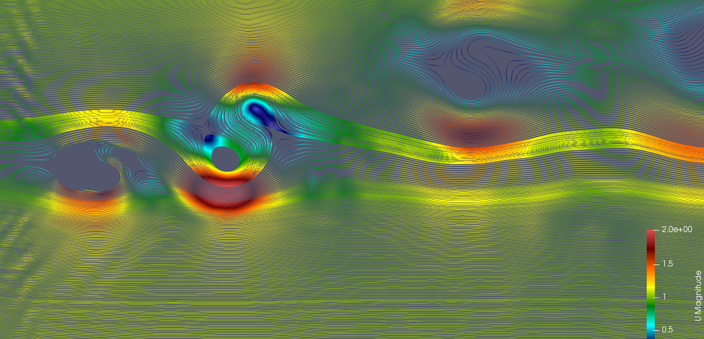
LZF
Articles9
Tags0
Categories0
2021快乐!集群搭建!

2021快乐!集群搭建!

2020对我来说是很特殊的一年,2021来了,总结一下两个电脑基于OpenMPI搭建的集群,希望2021也可以跑到飞起!

1.准备工作:
(1)两台同样版本ubuntu的虚拟机,将电脑主机连接在同一局域网下,windows命令输入win+R 输入cmd,打开终端,输入ipconfig,查看IPv4 地址,保证两个主机的IP地址前三位是相同的,例如:192.168.0.2和192.168.0.101。各个主机上的虚拟机网络模式设置为桥接模式,使用物理机局域网地址方便互相ping通。(若用Ubuntu系统搭建可以忽略前面部分)。Ubuntu终端输入ifconfig,出现如下界面:


两个节点测试是否能够ping通:(ping 的是inet的地址)


(2)修改两个节点的名称(例如node1,node2)
输入指令:vim /etc/hosts 添加如下两行


2.建立SSH无密码连接(两两之间连接)
(1)两台机子上均输入命令: sudo apt-get install ssh 进行安装ssh.
(2)尝试两个计算机的有密码登录,
node1键入: ssh node2
node2 键入: ssh node1


可见输入密码后均可互相ssh。

(3)免密登录步骤 :
第一步:在node1中通过ssh-keygen生成公钥私钥对。
键入: ssh-keygen (键入完一路按enter)


第二步:通过ssh-copy-id复制node1的公钥到node2


第三步:通过ssh-copy-id复制node2的公钥到node1(在node2上重复上两步)
尝试无密码ssh node1 成功:


(4)建立共享挂载文件夹:
node1和node2上均需要键入安装NFS:
sudo apt-get install nfs-kernel-server nfs-common
下载过后两个节点均建立共同挂载文件夹(mpicluster):
mkdir mcluster (此处切记不要sudo建立)
在node1节点上编辑/etc/exports文件(共享文件夹访问权限设置)
键入: sudo vi /etc/exports
在文件最下下添加如下一行:

/home/dyfluid/mcluster *(rw,sync,no_root_squash,no_subtree_check)


之后重新启动服务,键入:

sudo /etc/init.d/nfs-kernel-server restart

之后查看共享文件夹是否是mcluster,键入:

showmount -e

(5)将node2挂载在mpicluster文件夹下,node2下键入:
sudo mount -t nfs node1:/home/dyfluid/mcluster cluster
(node2节点每次重启后需运行此挂载命令)
(6)检查,在node1下mcluster文件夹中建立文件,在node2的mcluster中也能看见即为挂载成功!

3.建立openmpi并行计算环境
(1)虚拟机中of已经安装好openmpi,键入命令查看mpirun 是在哪里运行的:

which mpirun  

保证两个节点的mpirun运行环境皆是这个。
(3)在文件夹中下载of8和其ThirdParty,在两个节点上均进行编译,
在两台节点的~/.Bashrc中添加如下两行,将运行环境保证在挂载文件夹里:

source ~/mcluster/OpenFOAM-8/etc/bashrc
alias of8="source ~/mcluster/OpenFOAM-8/etc/bashrc"

注意:这个地方有大坑,一定一定要将
source ~/mcluster/OpenFOAM-8/etc/bashrc这一行添加到这个位置,不然没办法并行,这地方真的卡了我好久。。。


最后我们在挂载文件夹mcluster中需要运行的文件夹(这里面我用dambreak)之中放置配置文件,文件可以任意起名,例如:machines和hostfile,进而去设置调用每一个节点的核数,配置格式如下:


分块之后输入并行指令:
mpirun -hostfile machines -n 4 interFoam -parallel
或者:
mpirun -hostfile hostfile -n 4 interFoam -parallel
可见运行十分顺畅!

遇到的坑(随时更新)

遇到的坑(随时更新)

1.toposet要么在并行分块前设置要么就在分块后输入mpirun -np 24 topoSet -parallel,如果出现swap文件警告,删除swap文件

toposet,boxtoface

另外用toposet后处理捕捉一个面的拉格朗日液滴属性计算也太慢了吧!

of中涡量提取及张量操作运算符

of中涡量提取及张量操作运算符

提取涡量的方法

参考文献 [1] :http://xiaopingqiu.github.io/2016/05/22/QAndLambda/

(1). 用流线去封闭涡

(2). 速度梯度 ∇U 的二阶不变量 Q 的定义为

$Q=\frac{1}{2}\left(|\mathbf{W}|^{2}-|\mathbf{S}|^{2}\right)$
$\mathbf{W}=\frac{1}{2}\left(\nabla \mathbf{U}-(\nabla \mathbf{U})^{\mathrm{T}}\right)$
$|\mathbf{W}|=(\mathbf{W}: \mathbf{W})^{1 / 2}$
$\mathbf{S}=\frac{1}{2}\left(\nabla \mathbf{U}+(\nabla \mathbf{U})^{\mathrm{T}}\right)$
$|\mathbf{S}|=(\mathbf{S}: \mathbf{S})^{1 / 2}$

OpenFOAM 中 Q 的计算用的是下面的方法

volTensorField gradU(fvc::grad(U));

volScalarField Q
(
    IOobject
    (
        "Q",
        runTime.timeName(),
        mesh,
        IOobject::NO_READ,
        IOobject::AUTO_WRITE
    ),
    0.5*(sqr(tr(gradU)) - tr(((gradU)&(gradU))))
);

取Q>0的等值面

说到这里把张量运算符在of中的操作做一下总结

参考文献:[2] :《OpenFoam编程指南》.李东岳

of中湍流模型的植入(未完)

of中湍流模型的植入(未完)

Seaborn绘图总结(未完待续)

Seaborn绘图总结(未完待续)

圣诞快乐!

大数据量的绘图适合运用seaborn工具进行绘制,实验数据没备份丢失了,正好重新来一遍,做一个总结

绘图的数据源来自LPT生成数据的拉格朗日粒子,运行seaborn的环境是基于安装py3.7的miniconda。

1.

生成(csv)文件并读取文件

import pandas as pd

data = pd.read_csv('C:/Users/M/Desktop/U1.csv')

可以预览数据集

import seaborn as sns

sns.pairplot(data)

2.

sns.scatterplot(data.d,data.d)//单独绘制

# 只绘制核密度曲线,不绘制直返图,直方图hist=True,核密度曲线rug=True
ax = sns.distplot(data.w, rug=True, hist=True)

绘制核密度图

# shade参数决定是否填充曲线下面积
md = sns.kdeplot(data.d, shade=True, color="r")

绘制双变量核密度图

# 双变量密度图,相当于等高线图了
# shade 参数改用颜色深浅表示密度的大小,不过n不用,就真的是等高线了
nx = sns.kdeplot(data.w, data.u, shade=True,color="b")
g = sns.jointplot("w", "u", data=data, 
                    kind="kde", space=0,shade=True, color="g")
of中functionObjects函数的使用及Gnuplot

of中functionObjects函数的使用及Gnuplot

1.postProcess与functionObjects

OpenFoam分为两种后处理方法,一种是传统的postProcess方法,在求解后使用;另一种方法是在运行时进行处理的Co-processing,方法是在controlDict文件夹之中添加functionObjests,但有时可能事先忘记了在controlDict字典中定义functionObject,导致计算完毕后数据并未提取出来。OpenFOAM允许用户在求解计算完毕后执行functionObject,此时可以在controlDict文件中添加functionObject,然后利用命令提取数据。这里总结几个经常使用的后处理实用程序。
1.sampleDict文件
functionObject可以在求解过程中输出指定的物理量信息。当求解计算完毕后,可以选择使用Sampling获取特定位置物理信息,此时主要使用postProcess程序来实现。
输入postProcess -list来进行查看可实行后处理的目录
在system文件夹下添加sampleDict文件,文件格式例子如下

// * * * * * * * * * * * * * * * * * * * * * * * * * * * * * * * * * * * * //

type sets;

setFormat raw;

interpolationScheme cellPointFace;

fields
(
    U
);

sets
(

    l1
    {
        type            lineCellFace;
        axis            x;
        start           ( -1  0.5 0);
        end             ( 2  0.5 0);
    }

    l2
    {
        type            lineCellFace;
        axis            y;
        start           (0.5 -1 0);
        end             (0.5 2 0);
    }

);

// *********************************************************************** //

此文件指定两条箭头线,在在计算域中对线上进行取样```输入postProcess -func sampleDict -latestTime``命令进行对于最后一个时间步的采样工作,其结果会输出在postProcessing文件夹之中

建立gnuplot文件夹,在其下建立gnuplot_script文件去设置gnuplot脚本

set terminal qt 0//设置输出第一个窗口为0

#set multiplot layout 2,1

#set grid xtics//打网格
#set grid ytics
#set grid mxtics
#set grid mytics

set key left//图例放在左边,有left 和right两个选项;
set ylabel "Y centerline"//设置纵坐标
set xlabel "UX"//设置横坐标
plot 'gnuplot/UX_yline' u 2:1 w lp pt 7 title 'Ghia et al.','./postProcessing/sampleDict/50/l2_U.xy' u 2:1 pt 6 title 'Current solution'

#例子:plot  '.\line_rhoe1.xy' u 1:2  w lp lw 2 lt 2 pt 1 lc rgb "black" ,\
'.\line_rhoe2.xy' u 1:2  w l lw 2 lc rgb "black" 

#u 1:2 使用第一列数据为x轴,第二列数据为y轴 还可以进行运算 例如 u 1:($2)/($3)
#w lp 绘制数据点和数据线 w l 仅绘制数据线 w p仅绘制数据点
#lt/pt 2 点和线的绘制风格 lt0是虚线 可以使用dt命令设置其他点划线类型
# lc 线的颜色,同样会将该颜色设置给点
# 在gnuplot终端输入test可以快速查看所有电线风格


set terminal qt 1

set key default
set xlabel "X centerline"
set ylabel "UY"
plot 'gnuplot/UY_xline' u 1:2 w lp pt 7 title 'Ghia et al.','./postProcessing/sampleDict/50/l1_U.xy' u 1:3 pt 6 title 'Current solution'

#unset multiplot


pause -1

#    EOF

参考文献:[1]: https://blog.csdn.net/CloudBird07/article/details/106751196/

2.probesDict文件

FoamFile
{
    version     2.0;
    format      ascii;
    class       dictionary;
    object      probesDict;
}
// * * * * * * * * * * * * * * * * * * * * * * * * * * * * * * * * * * * * //
// 指定类型为probes
type probes;
// 指定需要提取的物理场
fields
(
    alpha.water
    U
    p_rgh
    p
);
// 取样点的坐标列表
probeLocations
(
    (0.292 0 0)
    (0.292 0.0240 0)
    (0.292 0.0480 0)
    (0.316 0.0480 0)
    (0.316 0.0240 0)
);

// * * * * * * * * * * * * * * * * * * * * * * * * * * * * * * * * * * * * 

之后在终端输入命令: postProcess -func probesDict
利用gnuplot进行绘制

3.几个functionObject

参考文献[2]: https://mp.weixin.qq.com/s/7t7IYaT0YCuJFhGeha0P6w

functionObject在controlDict字典文件中进行指定,且在预定义的时间点上执行操作。
functionObject在OpenFOAM求解计算的过程中可以实时修改。在OpenFOAM计算完毕后也可以执行
functionObject在controlDict字典文件中定义,打开controlDict文件。

FoamFile
{
    version     2.0;
    format      ascii;
    class       dictionary;
    object      controlDict;
}
// * * * * * * * * * * * * * * * * //

application     simpleFoam;
startFrom       startTime;
startTime       0;
stopAt          endTime;
endTime         2000;
deltaT          1;
writeControl    runTime;
writeInterval   50;
purgeWrite      100;
writeFormat     binary;   
writePrecision  8;
writeCompression off;
timeFormat      general;
timePrecision   6;
runTimeModifiable yes;

//下面为functionObject的定义
functions
{
forces_object
{
    // 指定类型为forces,必须项
    type forces;
    // 加载functionObject库
    functionObjectLibs ("libforces.so");

    // 指定数据输出频率
    writeControl   timeStep;
    writetInterval  1;

    // 激活functionObject对象
    enabled true;

    // 指定参与计算的边界,必须项
    patches ("wall_slat" "wall_airfoil" "wall_flap");

    //// 指定压力场与速度场的变量名称
    pName p;
    Uname U;

    // 参考密度值。它仅需要针对不可压缩的流进行定义。
    // 对于可压缩流,将使用计算的密度代替
    rho rhoInf;
    rhoInf 1.0;

    //// 指定力矩计算所需的旋转中心
    CofR (0 0 0);
}
// 关于forces的写法,可参阅文档:
/* https://cpp.openfoam.org/v8/classFoam_1_1functionObjects_1_1forces.html*/
///////////////////////////////////////////

forceCoeffs_object
{
    // 指定类型为力系数,该项为必选项
    type forceCoeffs;

    functionObjectLibs ("libforces.so");
    // 激活此对象
    enabled true;
    // 指定参与计算的边界名称,此项为必选项
    patches ("wall_slat" "wall_airfoil" "wall_flap");
    // 指定变量名称
    pName p;
    Uname U;

    // 仅用于不可压缩流动
    rho rhoInf;
    rhoInf 1.0;

    // 将数据写入到文件中
    log true;
    // 指定旋转中心坐标
    CofR (0.0 0 0);
    // 用于计算系数的参考值,4个均为必选项
    pitchAxis (0 0 1);    // 俯仰轴
    magUInf 1.0;    // 参考速度
    lRef 1;        // 用于力矩计算的参考长度
    Aref 1;        // 用于系数计算的参考面积

    // 指定数据的写入频率
    writeControl   timeStep;
    writeInterval  1;

    // 指定升力方向与阻力方向,必选项
    // 对于升力来讲,其值为攻角的三角函数(-sin,cos,0)
    // 对于阻力,其值为攻角的三角函数(cos,sin,0)
    // 注意角度换算为弧度
    liftDir     (0 1 0);       
    dragDir     (1 0 0);           
}   
////////////////////////////////////////////
minmaxdomain
{
    // 指定类型为fieldMinMax,必选项
    // 用于输出计算域内指定物理量的最大最小值
    type fieldMinMax;

    functionObjectLibs ("libfieldFunctionObjects.so");

    enabled true;
    // 指定计算物理场的分量,这里还可以指定magnitude
    mode component;
    // 指定数据写入频率
    writeControl timeStep;
    writeInterval 1;

    log true;
    // 指定需要输出的物理场
    fields (p U nuTilda nut k omega);
}
fieldAverage1
{
    // 指定类型fieldAverage,输出物理场的平均值
    type            fieldAverage;
    libs ( "libfieldFunctionObjects.so" );
    writeControl    writeTime;

    enabled         true;
    log             true;
    timeStart       100;
    // 下面指定需要输出的物理场,包括U,p及nut
    fields
    (
        U
        {
                mean        on;
                prime2Mean  on;
                base        time;
        }

        p
        {
                mean        on;
                prime2Mean  on;
                base        time;
        }

        nut
        {
                mean        on;
                prime2Mean  on;
                base        time;
        }
    );
}


//若直接包含外部定义的functionObject
#include "externalFunctionObject"
};

externalFunctionObject文件

{
    version     2.0;
    format      ascii;
    class       dictionary;
    object      functionObject;
}


//functions
//{
// 定义了监测点数据提取
probes_online
{
    type probes;
    functionObjectLibs ("libfieldFunctionObjects.so");
    enabled true;
    writeControl timeStep;
    writeInterval 1;

    probeLocations 
    (
        (1 0 0)
        (2 0 0)
        (2 0.25 0)
        (2 -0.25 0)
    );

    fields
    (  
        U
        p
    );

}

// 定义了涡量提取
vorticity
{
    type vorticity;
    functionObjectLibs ("libfieldFunctionObjects.so");
    enabled true;
    log    true;
    writeControl outputTime;  
}

有时可能事先忘记了在controlDict字典中定义functionObject,导致计算完毕后数据并未提取出来。OpenFOAM允许用户在求解计算完毕后执行functionObject,此时可以在controlDict文件中添加functionObject,然后利用命令:
name_of_the_solver -postProcess对参数进行输出
若定义了外在函数文件externalFunctionObject
则执行例如下命令:
interFoam-postProcess -dict system/externalFunctionObject –time 500:2000

El.Psy.Congroo!////

(以下为与自己相关的一些操作)

开始正题!

在of中用vof去模拟射流后处理是很难得出液滴直径PDF的(Probability Density Function概率密度分布函数),这个参数需要确定计算域里液滴的直径,而多相流直接数值模拟的方法没法通过设置计算的参数来确定液滴直径,这时候需要用几何捕捉的方法来确定液滴的属性。在OpenFoam中有效地从数值上检查整个雾化过程,欧拉方法和拉格朗日方法之间的转换是必要的。这种转变必须基于在欧拉VOF模拟的相场内检测到单独的流体粒子。结合检测,评估关于粒子的大小、位置和速度的信息。这个过程称为欧拉粒子检测。获得的信息然后可以作为初始值传递给拉格朗日框架中的点粒子。
从OpenFoam-v1612开始官方实现一个称为extractEulerianParticles的功能,这是一种基于2D耦合层的方法。具体的实现方法如下所示:
1.在system/controlDict 中添加如下

functions
{
    extractEulerianParticles1
    {
        // Mandatory entries
        type            extractEulerianParticles;
        libs            (fieldFunctionObjects);
        faceZone        collector;//你自己定义的面区域
        alpha           alpha.water;

        // Optional entries
        alphaThreshold  0.1;//相分数阈值
        nLocations      0;
        U               U;
        rho             rho;
        phi             phi;
        //minDiameter     1e-30;//可限定最大最小直径的阈值
        //maxDiameter     1e30;

        // Optional (inherited) entries
        writePrecision   6;
        writeToFile      true;
        useUserTime      false;

        region          region0;
        enabled         true;
        log             true;
        timeStart       0;
        timeEnd         1000;
        executeControl  timeStep;
        executeInterval 1;
        writeControl    writeTime;
        writeInterval   -1;
    }
}

此处需要注意的是,这个函数无法执行postProcess而且仅仅是在面上进行粒子的捕捉,如何放置这个面是2D耦合层需要考虑的棘手问题,故开发3D全场历遍液滴的算法是个解决的好办法。如果用这种方法去转化拉格朗日液滴是适合于几何结构上对称的射流的,来流雾化可能并不合适。但是对于处理某一个位置液滴直径的pdf还是一个非常好用的方法.

下面叙述一下toposet的用法:

FoamFile
{
    version     2.0;
    format      ascii;
    class       dictionary;
    object      topoSetDict;
}
// * * * * * * * * * * * * * * * * * * * * * * * * * * * * * * * * * * * * * //

// The topoSetDict comprises a list of actions to perform on different
// set types (cellSet, faceSet, pointSet, etc).
//
// Each action is a dictionary with e.g.
//     // Name of set
//     name    c0;
//
//     // type: pointSet/faceSet/cellSet/faceZoneSet/cellZoneSet
//     type    cellSet;
//
//     // action to perform on set. Two types:
//     // - require no source : clear/invert/remove
//     //       clear  : clears set or zone
//     //       invert : select all currently non-selected elements
//     //       remove : removes set or zone
//     // - require source    : new/add/subtract/subset
//     //       new    : create new set or zone from source
//     //       add    : add source to contents
//     //       subtract : subtract source from contents
//     //       subset : keeps elements both in contents and source
//     action  new;
//
// The source entry varies according to the type of set.
//
// In OpenFOAM 1806 and earlier, it was compulsory to use a 'sourceInfo'
// sub-dictionary to define the sources.
// In OpenFOAM 1812 and later, this sub-directory is optional, unless
// there would be a name clash (Eg, 'type' or 'name' appearing at both levels).
// In most cases, the source definitions have been adjusted to avoid such
// clashes.
//
// More detailed listing in the annotated topoSetSourcesDict

actions
(
    // Get all faces in cellSet
    {
        name    f0;
        type    faceSet;
        action  new;
        source  boxToFace;
        box     (0.099 0 0) (0.101 1 1);
    }

    // Determine inverse cellSet
    {
        name    fz1;
        type    faceZoneSet;
        action  new;
        source  setToFaceZone;
        faceSet f0;
    }
);

// ************************************************************************* //

这篇文章里写的很全,我不详细写了:参考文献 [3] ;http://www.xfy-learning.com/2020/05/19/OpenFOAM-topoSet/

梯度项在of中的植入

梯度项在of中的植入

of中压力梯度在周期性边界条件中的实现

参考文献:
[1] : https://www.cfd-china.com/topic/1992/cyclic%E5%91%A8%E6%9C%9F%E6%80%A7%E8%BE%B9%E7%95%8C%E6%9D%A1%E4%BB%B6/6
[2] : https://openfoam.org/release/2-2-0/boundary-conditions/
[3] : https://www.cfd-china.com/topic/2121/q-dns%E8%AE%A1%E7%AE%97%E6%A7%BD%E9%81%93%E6%B5%81%E9%81%87%E5%88%B0%E4%BA%86%E4%B8%80%E4%BA%9B%E9%97%AE%E9%A2%98-%E6%B1%82%E5%A4%A7%E7%A5%9E%E4%BB%AC%E6%8C%87%E7%82%B9
[4] : https://blog.csdn.net/CloudBird07/article/details/105102079

1.设置周期型边界条件需要使用cyclic边界条件并指定cyclic边界条件的类型,利用snappyHexMesh生成网格以及边界后进入ployMesh文件夹中编辑boundary文件,将想要设置为周期性边界条件的边界设置为cyclic并设置好他们的相邻边界,这里值得一提的是需要放大matchToTolerance的值方便之后createPatch的设定

    7
    (
        wall1
        {
            type            wall;
            inGroups        1(wall);
            nFaces          8232;
            startFace       9475455;
        }
        wall2
        {
            type            cyclic;
            inGroups        1(cyclic);
            nFaces          8232;
            startFace       9483687;
            //matchTolerance  1000;
            transform       none;
            neighbourPatch  wall3;
        }
        wall3
        {
            type            cyclic;
            inGroups        1(cyclic);
            nFaces          8232;
            startFace       9491919;
            // matchTolerance  1000;
            transform       none;
            neighbourPatch  wall2;
        }
        wall4
        {
            type            wall;
            inGroups        1(wall);
            nFaces          8232;
            startFace       9500151;
        }
        wall5
        {
            type            cyclic;
            inGroups        1(cyclic);
            nFaces          34548;
            startFace       9508383;
            // matchTolerance  1000;
            transform       none;
            neighbourPatch  wall6;
        }
        wall6
        {
            type            cyclic;
            inGroups        1(cyclic);
            nFaces          34548;
            startFace       9542931;
            //matchTolerance  1000;
            transform       none;
            neighbourPatch  wall5;
        }
        BALL
        {
            type            wall;
            inGroups        1(wall);
            nFaces          152712;
            startFace       9577479;
        }
    )

下一步就是建立createPatchDict文件对周期性边界条件进行设置

//       with transformations (i.e. cyclics).
pointSync false;

// Optional: Write cyclic matches into .obj format; defaults to false.
writeCyclicMatch  false;

// Patches to create.
patches
(
    {
    // Name of new patch
        name wall2;

        // Dictionary to construct new patch from
        patchInfo
        {
            type cyclic;
            neighbourPatch wall3;

            // Optional: explicitly set transformation tensor.
            // Used when matching and synchronising points.
            //transform rotational;
            //rotationAxis (1 0 0);
            //rotationCentre (0 0 0);
            // transform translational;
            // separationVector (1 0 0);

            // Optional non-default tolerance to be able to define cyclics
            // on bad meshes
            // matchTolerance 1E-2;
        }

        // How to construct: either from 'patches' or 'set'
        constructFrom patches;

        // If constructFrom = patches : names of patches. Wildcards allowed.
        patches (wall2);

        // If constructFrom = set : name of faceSet
        //set f0;
    }
    {
        // Name of new patch
        name wall5;

        // Dictionary to construct new patch from
        patchInfo
        {
            type cyclic;
            neighbourPatch wall6;

            // Optional: explicitly set transformation tensor.
            // Used when matching and synchronising points.
            //transform rotational;
            //rotationAxis (1 0 0);
            //rotationCentre (0 0 0);
            // transform translational;
            // separationVector (1 0 0);
        }

        // How to construct: either from 'patches' or 'set'
        constructFrom patches;

        // If constructFrom = patches : names of patches. Wildcards allowed.
        patches (wall5);

        // If constructFrom = set : name of faceSet
    //set f0;
    }
);

注意此处有坑:设置patch的边界一定要设置为你在boundary文件里最先设置为cyclic的边界。
执行creatPatch与checkMesh命令实现周期性边界条件设置。
2.of中周期性边界条件的压力梯度实现有两种方法:
一种是在初始边界条件上运用fixedJump方法,设置两个边界的压差实现压力梯度驱动,这种方法最为简单。

inlet
    {
        type               fixedJump;
        patchType       cyclic;
        jump            uniform -151;
        value           $internalField;

    }

    outlet
    {
        type            fixedJump;
        patchType       cyclic;
        value           $internalField;

    }

另外一种方法是对动量方程实现修改,添加一个压力梯度的源项,其实现方法如下:
(1)首先定义一个基于原求解器的自定义求解器,方法详见: https://www.bilibili.com/video/av75230449/
在creatFields文件中添加压力梯度场:

volVectorField pGrad 
( 
    IOobject 
    ( 
        "pGrad", 
        runTime.timeName(), 
        mesh, 
        //IOobject::MUST_READ, 
        IOobject::NO_READ, 
        IOobject::AUTO_WRITE 
    ), 
    mesh, 
    //Zero 
    //vector(500, 0, 0) 
    dimensionedVector("pGrad",dimensionSet(1, -2, -2, 0, 0),vector(-500,0,0)) 
); 

此处值得注意的是定义的场为矢量场,且他的单位应该是压力梯度的单位,这里设置它的数值为x方向的-500;
之后在UEqn.H求解动量方程文件中添加源项:

MRF.correctBoundaryVelocity(U); 

    fvVectorMatrix UEqn 
    ( 
            fvm::ddt(rho, U) + fvm::div(rhoPhi, U) 
        + MRF.DDt(rho, U) 
        + turbulence->divDevRhoReff(rho, U) 
        + fvm::Sp(rho*coupling.damping(), U) 
        + fvm::Su(rho*coupling.source(), U) 
        == 
            fvOptions(rho, U)-pGrad 
    ); 

    UEqn.relax(); 

实现之后执行wmake进行重新编译就可实现每个网格上均匀压力梯度驱动的求解器了

3.那么同样是体积力,在设置重力文件中添加数值是否和以上添加压力梯度的方法起到一样的效果呢,答案是否定的:

fvOptions.constrain(UEqn); 

    if (pimple.momentumPredictor()) 
    { 
        solve 
        ( 
            UEqn 
        == 
            fvc::reconstruct 
            ( 
                ( 
                    mixture.surfaceTensionForce() 
                - ghf*fvc::snGrad(rho) 
                - fvc::snGrad(p_rgh) 
                ) * mesh.magSf() 
            ) 
        ); 

        fvOptions.correct(U); 
    } 

我们可以看到方程中重力项的实现是- ghf*fvc::snGrad(rho),ghf定义如下:

new surfaceScalarField
(
    "ghf",
    (gFluid[i] & fluidRegions[i].Cf()) - ghRef
)

其中gFluid[i]返回了通过字典(constant/g)读取得到的重力加速度项,fluidRegions[i].Cf()返回了当前网格表面的面心矢量,ghRef是给定的相对重力加速度,一般为0。综上所述,openFOAM中的重力的表达式为:$\vec{G}=-(\vec{g} \cdot \vec{s}) \nabla \rho$
其中$\vec{S}$是待求点的位置矢量,这显然与方程1使用的重力表达式相差很大,接下来我们就一步一步推导这个结果。
首先明确,在涉及到重力的求解器中,其求解的压力p并不是总压P,而是动压,即:$P=p+\rho \vec{g} \cdot \vec{s}$
之所以要这样处理是为了方便用户设置初场,大家可以设想最简单的溃坝算例,如果直接对总压设置初场,那我们要设置的则是一个梯形的压力分布,计算域的y坐标越高其净水压强就越大,而如果我们拆分成动压和静压的形式,就可以直接设置初场为0了。在动量方程中,我们存在对总压的压力梯度项,将总压拆成静压和动压即可得到:

$\nabla P=\nabla(p+\rho \vec{g} \cdot \vec{s})=\nabla p+\nabla(\rho \vec{g} \cdot \vec{s})=\nabla p+(\vec{g} \cdot \vec{s}) \nabla \rho+\rho \nabla(\vec{g} \cdot \vec{s})$

$\nabla(\vec{g} \cdot \vec{s})=\nabla(g y)=\left(\frac{\partial(g y)}{\partial x}, \frac{\partial(g y)}{\partial y}, \frac{\partial(g y)}{\partial z}\right)=(0, g, 0)=\vec{g}$

$\nabla P=\nabla p+(\vec{g} \cdot \vec{s}) \nabla \rho+\rho \nabla(\vec{g} \cdot \vec{s})=\nabla p+(\vec{g} \cdot \vec{s}) \nabla \rho+\rho \vec{g}$

得到Open foam中动量方程

$\rho \frac{\partial \vec{u}}{\partial t}+\rho \nabla(\vec{u} u)=\nabla(\mu \nabla \vec{u})-\nabla p-(\vec{g} \cdot \vec{s}) \nabla \rho$

故确实是of中重力相起体积力源项的作用,但是返回的是$(\vec{g} \cdot \vec{s}) \nabla \rho$和增加压力梯度是同样的效果单位也是(1,-2,-2,0,0,0,0),但是是无法通过直接给g的数值来达到添加压力梯度的条件的。

测试

测试

测试标题封面,测试插入射流图片,测试输入公式

$\frac{\partial \rho \mathbf{U}}{\partial t}+\nabla \cdot(\rho \mathbf{U} \mathbf{U})-\nabla \cdot \tau=-\nabla p+\rho \mathbf{g}+\mathbf{F}$
$\frac{\partial \rho}{\partial t}+\nabla \cdot(\rho \mathbf{U})=0$
$\nabla \cdot \mathbf{U}=0$

HelloWorld

HelloWorld

有道无术,术尚可求也,有术无道,止于术

CFD小白用于做一些自己的总结,顺便提升一下自己写文章的水平,欢迎批评讨论指正

wx:13080703991